---
title: Coupled Free-Flow and Porous Media Flow Models in DuMu^x^
---
# Motivation
## Environmental and Agricultural Issues
:::::: {.columns}
::: {.column width=65%}
<img src="img/FFPM_radiation.gif"/>
<small>Fig.1 - Evaporation of soil water (Heck et al. (2020))<sup>1</sup></small>
:::
::: {.column width=35%}
* Evaporation of soil water
* Soil salinization
* Underground storage (e.g. CO2, atomic waste)
:::
::::::
## Technical Issues
:::::: {.columns}
::: {.column width=50%}

<small style="text-align: center;">Fig.2 - Filter (Schneider et al. (2023))<sup>2</sup></small>
:::
::: {.column width=50%}
* Fuel cells
* Filters (e.g. air)
* Heat exchangers (e.g. CPU cooling)
:::
::::::
## Biological Issues
:::::: {.columns}
::: {.column width=28%}
<img src="img/FFPM_braintissue.png"/>
<small>Fig.3 - Brain tissue (Koch et al. (2020))<sup>3</sup></small>
:::
::: {.column width=50%}
* Brain tissue
* Leaf structure
:::
::::::
# Model Overview
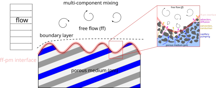
## Conceptual Physical Model
{style="width: 80%; align: left;"}
<figcaption align = "center">
<font size = "2">
Fig.5 - Exchange processes at the free-flow porous-medium interface at different scales (Photo: Martin Schneider)
</font>
</figcaption>
## Mathematical Model
:::::: {.columns}
::::: {.column width=15%}

:::::
::::: {.column width=85%}
**Free Flow:**
<font size=5.9>
* Stokes / Navier-Stokes / RANS
* 1-phase, n-components, non-isothermal
</font>
**Interface conditions:**
<font size=5.9>
* no thickness, no storage, local thermal equilibrium
* continuity of fluxes and state variables
</font>
**Porous media:**
<font size=5.9>
* Darcy / Forchheimer
* m-phases, n-components, non-isothermal
</font>
:::::
::::::
## Numerical Model
<img src=img/FFPM-numericalmodel.png width="25%">
<figcaption align = "center">
<font size = "2">
Fig.6 - Discretization scheme (Fetzer (2018))<sup>4</sup>
</font>
</figcaption>
# Exercises
## Exercise Tasks
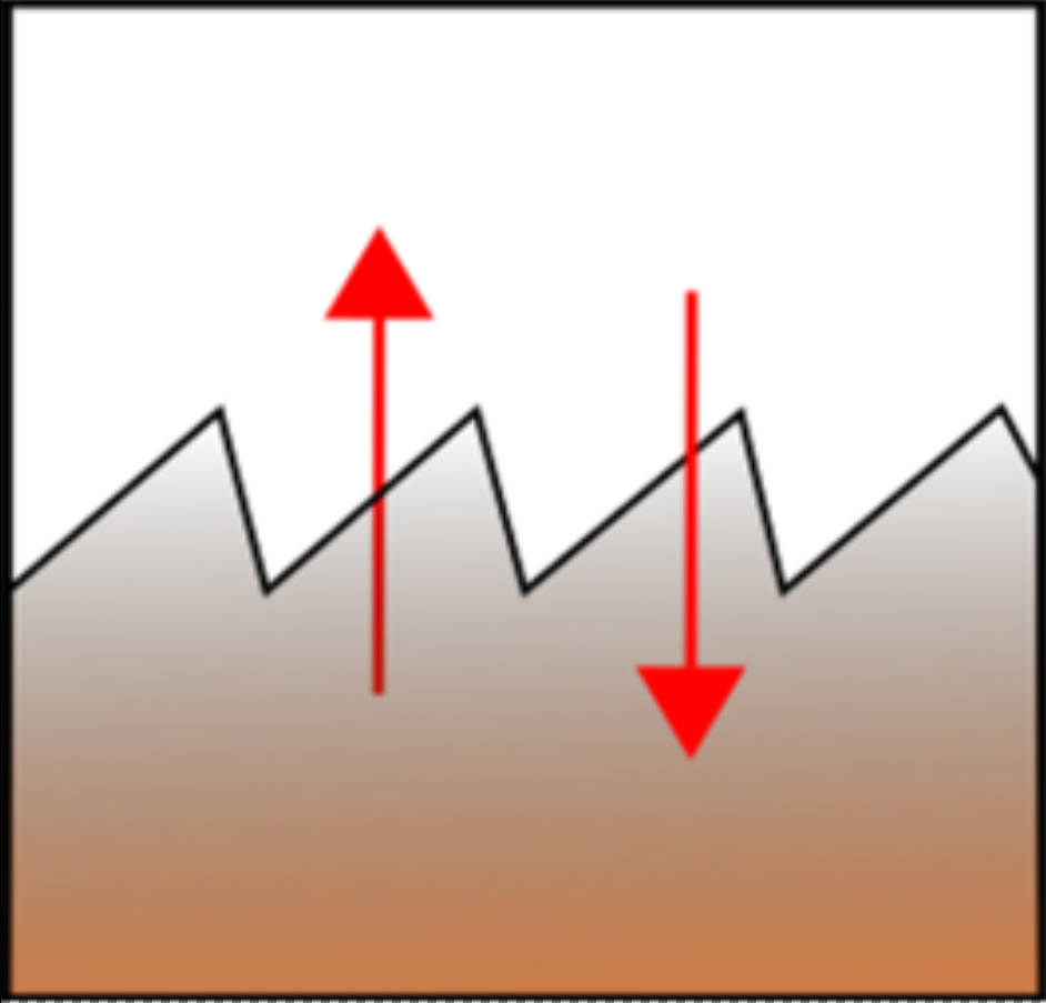
1. __Interface__
- Change flow direction
- Introduce slip condition
- Change shape of interface
2. __Porous Medium Model__
- Use 2-phase multicomponent model
- Investigate and export water loss and visualize it
3. __Free-Flow region__
- Introduce a turbulence model
- Use symmetry boundary conditions
- Apply grid refinement towards interface
# <small> Supplementary Material</small> </br>Model equations
## Eqs - Free Flow
:::::: {.columns}
::::: {.column width=15%}

:::::
::::: {.column width=85%}
* Momentum balance (Navier-Stokes equation)
$$
\frac{\partial \left(\rho_g \textbf{v}_g\right)}{\partial t} + \nabla \cdot (\rho_g \textbf{v}_g \textbf{v}_g^T) - \nabla \cdot \mathbf{\tau}_g +\nabla \cdot (p_g\textbf{I})- \rho_g \textbf{g} = 0
$$
* Component mass balance
$$
\frac{\partial \left(\rho_g X^\kappa_g\right)}{\partial t} + \nabla \cdot \left( \rho_g X^\kappa_g \textbf{v}_g + \mathbf{j}_{\text{diff}}^\kappa\right) - q^\kappa = 0
$$
:::::
::::::
## Eqs - Free Flow
:::::: {.columns}
::::: {.column width=15%}

:::::
::::: {.column width=85%}
* Energy balance
$$
\begin{aligned}
\frac{\partial (\rho_g u_g) }{\partial t} + \nabla \cdot (\rho_g h_g \textbf{v}_g) &+ \sum_{\kappa} {\nabla \cdot (h_g^\kappa \textbf{j}_{\text{diff}}^\kappa)} \\ &- \nabla \cdot (\lambda_{g} \nabla T) = 0
\end{aligned}
$$
:::::
::::::
## Eqs - Porous Medium Flow
:::::: {.columns}
::::: {.column width=15%}

:::::
::::: {.column width=90%}
* Darcy velocity (momentum balance)
$$
\textbf{v}_\alpha = - \frac{k_{r,\alpha}}{\mu_\alpha} K \left(\nabla p_\alpha - \rho_\alpha \textbf{g}\right)
$$
* Component mass balance
$$
\sum\limits_{\alpha \in \{\text{l, g} \}} \left(\phi \frac{\partial \left(\rho_\alpha S_\alpha X_\alpha^\kappa\right)}{\partial t } + \nabla \cdot \rho_\alpha X_\alpha^\kappa \textbf{v}_\alpha + \nabla \cdot \mathbf{j}_{\text{diff}}^\kappa\right) = 0
$$
:::::
::::::
## Eqs - Porous Medium Flow
:::::: {.columns}
::::: {.column width=15%}

:::::
::::: {.column width=90%}
* Total energy balance
$$
\begin{aligned}
\sum\limits_{\alpha \in \{\text{l, g} \}} &\left(\phi\frac{\partial \left(\rho_\alpha S_\alpha u_\alpha\right)}{\partial t} + \nabla \cdot \left(\rho_\alpha h_\alpha \textbf{v}_\alpha \right)\right) \\
&+ \left(1-\phi\right) \frac{\partial \left(\rho_s c_{p,s}T\right)}{\partial t} - \nabla\cdot \left(\lambda_{pm} \nabla T \right) = 0
\end{aligned}
$$
:::::
::::::
## Eqs - Coupling Conditions
:::::: {.columns}
::::: {.column width=15%}
:::::
::::: {.column width=85%}
* Continuity of total mass flux
$$
[(\rho_g \textbf{v}_g) \cdot \textbf{n}]^{\text{ff}} = - [(\rho_g \textbf{v}_g + \rho_w \textbf{v}_w) \cdot \textbf{n}]^{\text{pm}}
$$
* Continuity of component flux
$$
\begin{aligned}
&\left[(\rho_g X_g^\kappa \textbf{v}_g + \textbf{j}_{\text{diff}^\kappa}) \cdot \textbf{n}\right]^{\text{ff}} = \\&- \left[\left( \sum_{\alpha} (\rho_{\alpha} X_{\alpha}^\kappa \textbf{v}_\alpha + \textbf{j}^\kappa_{\text{diff}, \alpha})\right) \cdot \textbf{n}\right]^{\text{pm}}\,
\end{aligned}
$$
:::::
::::::
## Eqs - Coupling Conditions
:::::: {.columns}
::::: {.column width=15%}
<img src="img/FFPM-couplingsymbol.png">
<figure>
<img src="img/FFPM-BJS.png" alt="BJS Symbol">
<figcaption style="font-size: small; text-align: left;">Beaver-Joseph slip condition</figcaption>
</figure>
:::::
::::: {.column width=85%}
* Momentum condition in normal direction
$$
\left[((\rho_g \textbf{v}_g \textbf{v}_g^T - \mathbf{\tau}_g + p_g\textbf{I}) \textbf{n} )\right]^{\text{ff}} = \left[(p_g\textbf{I})\textbf{n}\right]^{\text{pm}}\,
$$
* Momentum condition in tangential direction
$$
\begin{aligned}
\left[\left(- \textbf{v}_g - \frac{\sqrt{(\textbf{K}\textbf{t}_i)\cdot \textbf{t}_i}}{\alpha_{\mathrm{BJ}}} (\nabla \textbf{v}_g + \nabla \textbf{v}_g^T)\textbf{n} \right) \cdot \textbf{t}_i \right]^{\text{ff}} = 0\, , \\
\quad i \in \{1, .. ,\, d-1\}\,
\end{aligned}
$$
:::::
::::::
## Eqs - Coupling Conditions
:::::: {.columns}
::::: {.column width=15%}

:::::
::::: {.column width=85%}
* Continuity of energy fluxes
<font size = "5">
$$
\begin{aligned}
\left[\left(\rho_g h_g \textbf{v}_g + \sum_i h_g^\kappa \textbf{j}_{\text{diff},g}^\kappa - \lambda_{g} \nabla T\right)\cdot \textbf{n}\right]^{\text{ff}} =\\ - \left[\left( \sum_\alpha (\rho_\alpha h_\alpha \textbf{v}_\alpha + \sum_\kappa h_\alpha^\kappa \textbf{j}_{\text{diff},\alpha}^\kappa) - \lambda_{\text{pm}}\nabla T\right)\cdot \textbf{n}\right]^{\text{pm}}\,
\end{aligned}
$$
</font>
:::::
::::::
# <small> Supplementary Material</small> </br>Example: Soil-Water Evaporation
## Example: Soil-Water Evaporation
:::::: {.columns}
::::: {.column width=50%}
<img src=img/FFPM-TurbulentBoundaryLayer.png width="80%">
:::::
::::: {.column width=50%}
<img src=img/FFPM-SoilWaterEvapField.png width="80%">
<figcaption align = "center">
<font size = "2">
Fig.7 - Evaporation in the water cycle (Shahraeeni et al. (2012))<sup>5</sup>
</font>
</figcaption>
:::::
::::::
## Example: Soil-Water Evaporation
<img src=img/FFPM-evapStages.png width="60%">
<figcaption align = "center">
<font size = "2">
Fig.8 - Different evaporation stages (Or et al.(2013))<sup>6</sup>
</font>
</figcaption>
## Example: Simple Evaporation Setup
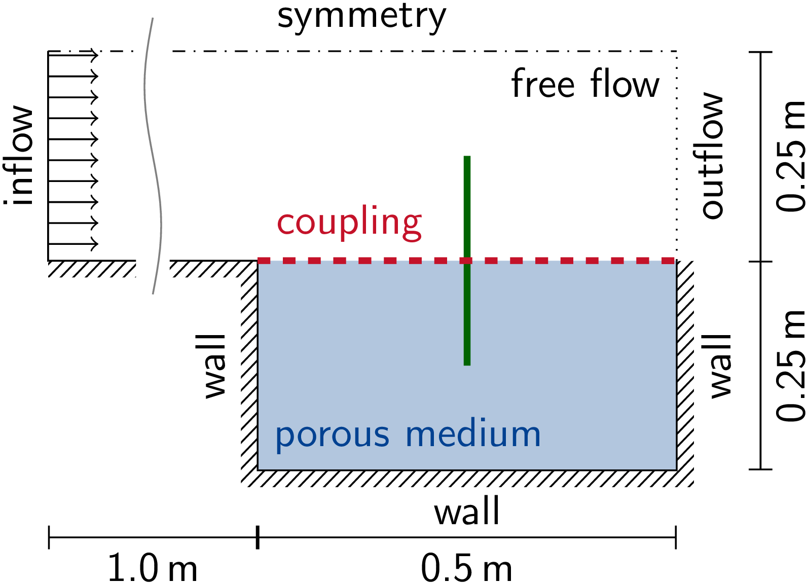{style="width: 60%; margin: auto; float: left;"}
<font size = "2">
Tab1: Input parameter
</font>
<font size = "5">
| Parameter | Value |
|:----------------------------|--------------:|
| $\textbf{v}_g^{ff}$ [m/s] | (3.5,0)$^T$ |
| $p_g^{ff}$ [Pa] | 1e5 |
| $X_g^{w,ff}$ [-] | 0.008 |
| $T^{ff}$ [K] | 298.15 |
| $p_g^{pm}$ [Pa] | 1e5 |
| $S_l^{pm}$ [-] | 0.98 |
| $T^{pm}$ [K] | 298.15 |
</font>
<figcaption align = "left">
<font size = "2">
Fig.9 - Model setup (Fetzer (2018))<sup>4</sup>
</font>
</figcaption>
## Example: Results

<figcaption align = "center">
<font size = "2">
Fig.10 - Results: Evaporation from a simple setup (Fetzer (2018))<sup>4</sup>
</font>
</figcaption>
# References
##
<font size = "5">
1. Heck, K., Coltman, E., Schneider, J. and Helmig, R. (2020). Influence of radiation on evaporation rates: A numerical analysis. Water Resources Research, 56, e2020WR027332. https://doi.org/10.1029/2020WR027332
2. Schneider, M., Gläser, D., Weishaupt, K., Coltman, E., Flemisch, B. and Helmig, R. (2023). Coupling staggered-grid and vertex-centered finite-volume methods for coupled porous-medium free-flow problems. Journal of Computational Physics. 112042. https://doi.org/10.1016/j.jcp.2023.112042.
3. Koch, T., Flemisch, B., Helmig, R., Wiest, R. and Obrist, D. (2020). A multiscale subvoxel perfusion model to estimate diffusive capillary wall conductivity in multiple sclerosis lesions from perfusion MRI data. Int J Numer Meth Biomed Engng. 36:e3298. https://doi.org/10.1002/cnm.
4. Fetzer, Thomas: Coupled Free and Porous-Medium Flow Processes Affected by Turbulence and Roughness – Models, Concepts and Analysis, Universität Stuttgart. - Stuttgart: Institut für Wasser- und Umweltsystemmodellierung, 2018
5. Shahraeeni, E., Lehmann, P. and Or, D. (2012). Coupling of evaporative fluxes from drying porous surfaces with air boundary layer: Characteristics of evaporation from discrete pores. Water Resources Research. 48. 9525-. 10.1029/2012WR011857.
6. Or, D., Lehmann, P., Shahraeeni, E. and Shokri, N. (2013), Advances in Soil Evaporation Physics—A Review. Vadose Zone Journal, 12: 1-16 vzj2012.0163. https://doi.org/10.2136/vzj2012.0163
</font>