Biomineralization
We simulate microbially-induced calcite precipitation in a vertical sand-column. The problem is considered radially-symmetric so that a one-dimensional problem can be simulated.
The main points illustrated in this example are
- solving a reactive transport model including
- biofilm growth
- mineral precipitation and dissolution
- changing porosity and permeability
- using complex fluid and solid systems
- setting a complex time loop with checkpoints, reading the check points from a file
- set complex injection boundary conditions, reading the injection types from a file
Table of contents. This description is structured as follows:
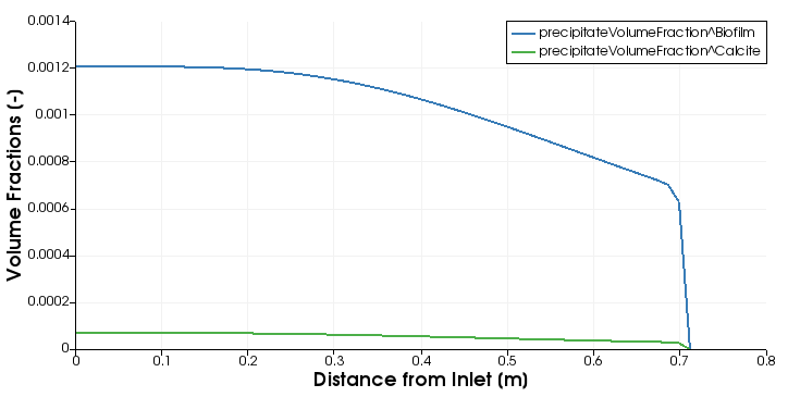
Result. The result will look like below. You see the volume fractions of the solid components after 100000s over the column.
Problem set-up
A vertical, sand-filled column is biomineralized by repeated injections of various aqueous solutions from its bottom end. The setup will be explained in more detail in Part 3: Example Setup. For more information, see the description of column experiment D1 in Section 4.2 of @Hommel2016.
What is microbially-induced calcite precipitation?
Microbially-induced calcite precipitation (MICP) is an engineering technology for targeted biomineralization. It can be used in the context of sealing possible leakage pathways of subsurface gas or oil reservoirs as well as other applications. The governing processes are two-phase multi-component reactive transport including precipitation and dissolution of calcite, as well as biomass-related processes:
- attachment of biomass to surfaces,
- detachment of biomass from a biofilm,
- growth and decay of biomass.
Additionally, the reduction in porosity and permeability has to be considered. This results from the presence of the solid phases biofilm and calcite in the pore space.
In subsurface applications, MICP is typically associated with a reduction of porosity, which, even more importantly, corresponds to a reduction of permeability. MICP can be used to alter hydraulic flow conditions, for example, by filling highly permeable pathways such as fractures, faults, or behind-casing defects in boreholes within a geological formation, e.g. @Phillips2013a.
The bacterium Sporosarcina pasteurii expresses the enzyme urease that catalyzes the hydrolysis reaction of urea (CO(NH2)2) into ammonia (NH3) and carbon dioxide (CO2):
\mathrm{CO(NH_2)_2} + 2\mathrm{H_2O} \xrightarrow{urease}
2\mathrm{NH_{3}} + \mathrm{H_2CO_{3}}.
\tag{1}
Aqueous solutions of ammonia become alkaline until the equilibrium of ammonium and ammonia is reached. Thus, the ureolysis reaction leads to an increase in pH until the pH is equal to the pKa of ammonia. This shifts the carbonate balance in an aqueous solution toward higher concentrations of dissolved carbonate. Adding calcium to the system results then in the precipitation of calcium carbonate:
\mathrm{CO_{3}^{2-}} + \mathrm{Ca^{2+}} \longrightarrow \mathrm{CaCO_3 \downarrow}.The resulting overall MICP reaction equation is:
\mathrm{CO(NH_2)_2} + 2\mathrm{H_2O} + \mathrm{Ca^{2+}} \xrightarrow{urease}
2\mathrm{NH_{4}^{+}} + \mathrm{CaCO_{3}} \downarrow.
In a porous medium, biofilm growth, fluid dynamics, and reaction rates are strongly interacting. A pore-scale sketch of the most important processes of MICP is shown in Fig.2.

A major difficulty for practical engineering applications of MICP is the predictive planning of a scenario and its impact. While the basic chemistry and the flow processes are known, it is mainly the quantitative description of the influence of the biofilm and the developing precipitates on hydraulic parameters that poses challenges to achieving predictability. More details on modeling biomineralization are given in Part 1: Model Concept.
The code documentation
In the following, we take a closer look at the source files for this example. The setup is rather complex in comparison to the other examples. We will discuss the different parts of the code in detail subsequently.
└── biomineralization/
    ├── CMakeLists.txt          -> build system file
    ├── main.cc                 -> main program flow
    ├── params.input            -> runtime parameters
    ├── injections.dat          -> runtime injection strategy input file
    ├── properties.hh           -> compile time settings for the simulation
    ├── problem.hh              -> boundary & initial conditions for the simulation
    ├── spatialparams.hh        -> parameter distributions for the simulation
    └── material/               -> components, fluid- and solidsystems
        ├── components/
        │   ├── biofilm.hh
        │   └── suspendedbiomass.hh
        ├── fluidsystems/
        │   ├── biominsimplechemistry.hh
        │   └── icpcomplexsalinitybrine.hh
        ├── solidsystems/
        │   └── biominsolids.hh
        └── co2tableslaboratory.hh
In order to define a simulation setup in DuMux, you need to implement compile-time settings,
where you specify the classes and compile-time options that DuMux should use for the simulation.
Moreover, a Problem class needs to be implemented, in which the initial and boundary conditions
are specified. Finally, spatially-distributed values for the parameters required by the used model
are implemented in a SpatialParams class.
Part 1 discusses the mathematical model in more detail.
Part 2 takes a close look at the main file.
main.cc controlling the simulation, and containing the time loop management,
A special feature of this example, which might be interesting also for non-biomineralization modelers,
is that it uses the class CheckPointTimeLoop extensively to set the injections of the various consecutive
biomineralization solution injections based on a separate input file injections_checkpoints.dat.
Similar strategies might be useful when simulating experimental setups with boundary conditions changing over time.
Part 3 takes a close look at the problem set-up.
problem.hh featuring the reactive source and sink terms discussed in the model concept and the time-dependent injection boundary conditions, and
spatialparams.hh with the spatially distributed parameters, most importantly the porosity and permeability changing due to the reactions.
A special feature of this example, which might be interesting also for non-biomineralization modelers,
is that problem.hh, determines the Neumann boundary condition, more specifically which type of solution is currently injected, (the injectionType_) based on a separate input file injections_type.dat.
Similar strategies might be useful when simulating experimental setups with boundary conditions changing over time.
Part 4 discusses the code concerned with the fluid (files in the folder material/),
especially the multi-component fluidsystems.
The CO2 properties are stored in the CO2 tables in the subfolder material (co2tableslaboratory.hh,co2valueslaboratory.inc).
Part 5 discusses the code concerned with the solid properties (files in the folder material/),
especially the multi-component solidsystems and variable solid volume fractions.
Part 1: Model concept
| ➡️ Click to continue with part 1 of the documentation |
|---|
Part 2: Main file
| ➡️ Click to continue with part 2 of the documentation |
|---|
Part 3: Simulation setup
| ➡️ Click to continue with part 3 of the documentation |
|---|
Part 4: Specific fluid material files
| ➡️ Click to continue with part 4 of the documentation |
|---|
Part 5: Specific solid material files
| ➡️ Click to continue with part 5 of the documentation |
|---|