Exercise Biomineralization (DuMuX Course)

The aim of this exercise is to get a first glimpse at the DuMu^x way of implementing mineralization and reaction processes. In the scope of this exercise, the setting of boundary conditions is revisited and a new reaction term is implemented.

Problem set-up

The domain has a size of 20 x 15 m and contains a sealing aquitard in the middle. The aquitard is interrupted by a "fault zone" and thereby connects the upper drinking water aquifer and the lower CO₂-storage aquifer. Initially, the domain is fully saturated with water and biofilm is present in the lower CO₂-storage aquifer. Calcium and urea are injected in the upper drinking water aquifer by means of a Neumann boundary condition. The remaining parts of the upper boundary and the entire lower boundary are modelled with Neumann no-flow conditions, while on the right-hand side a Dirichlet boundary conditions is assigned, which fixes there the initial values.

Disclaimer: Please note, that this is not a realistic scenario. No one would think of storing gaseous CO₂ in this subcritical setting.

Preparing the exercise

• Navigate to the directory dumux-course/exercises/exercise-biomineralization

1. Getting familiar with the code

Locate all the files you will need for this exercise

• The main file : main.cc
• The input file: params.input
• The problem file : biominproblem.hh
• The properties file: properties.hh
• The spatial parameters file: biominspatialparams.hh

Furthermore you will find the following folders:

• chemistry: Provides a way to formulate reactions via source/sink terms.
• components: Provides some additional components, e.g. biofilm and urea.
• fluidsystems: Stores headers containing data/methods on fluid mixtures of pure components.
• fluidmatrixinteractions: Stores headers containing methods on fluid-solid interactions, i.e. the permeability law.
• solidsystems: Stores headers containing data/methods on solid mixtures of the components.

To find out more on chemistry, components, fluidsystems, fluidmatrixinteractions, and solidsystems implementations, you may have a look at the folder dumux/material.

Special note on solidsystems: There are two types of solid components: reactive and inert. For each reactive component, one mass balance is solved. The inert components compose the "unchanging" (inert) rock matrix.

2. Implement a chemical equation

In the following, the basic steps required to set the new chemical equation are outlined. Here, this is done in the chemistry folder in the prepared file: simplebiominreactions.hh within the function reactionSource(). Please be aware, that the chemistry file already provides some convenience functions (e.g. moleFracToMolality()).

Task

Add a kinetic reaction by first calculating the current mass of available biofilm. Note that the density and volume fraction of biofilm are already defined for you.

\displaystyle mass_{biofilm} = \rho_{biofilm} * \phi_{biofilm}

Next, we want to implement the rate of ureolysis. This can be done with the following simplified equation:

\displaystyle r_{urea} = k_{urease} * Z_{u,b} * m_{urea} / (K_{urea} + m_{urea}),

where \displaystyle r_{urea} is the rate of ureolysis, \displaystyle k_{urease} the urease enzyme activity, \displaystyle m_{urea} the molality of urea and \displaystyle K_{urea} the half-saturation constant for urea for the ureolysis rate.

Note, that the urease concentration \displaystyle Z_{u,b} has a kinetic term of urease production per biofilm :

\displaystyle Z_{u,b} = k_{u,b} * mass_{biofilm}

For the sake of simplicity, we consider the rate of calcite precipitation \displaystyle r_{prec} to be equal to the rate of ureolysis \displaystyle r_{urea}:

\displaystyle r_{prec} = r_{urea}

Note that this assumption is a substantial simplification of the geochemistry, representing a state after sufficient ureolysis has occurred to raise the pH enough to initiate calcite precipitation. For a more detailed geochemistry, the exact speciation of inorganic carbon into \mathrm{CO_{2}}, \mathrm{H_{2}CO_{3}}, \mathrm{HCO_{3}^{-}}, and \mathrm{CO_{3}^{2-}} would have to be considered. This would require to calculate activity coefficients and solve the coupled laws of mass actions of the dissociation reaction of the inorganic carbon species as well as the one for ammonia and ammonium, which are all coupled by the solution pH, or rather the occurrence of \mathrm{H^{+}} in all those reactions. As such, this would require to solve a coupled system of equations to balance the geochemistry. Finally, the product of the activities of carbonate and calcium would need to be compared to the calcite solubility product to determine the saturation state of the solution with respect to calcite and to ultimately calculate the precipitation rate of calcite \displaystyle r_{prec}

The last step is defining the source term \displaystyle q for each component based on the now defined reaction rates \displaystyle r_{urea} and \displaystyle r_{prec} according to the chemical reaction equations:

\displaystyle \mathrm{CO(NH_{2})_{2} + 2 H_{2}O \rightarrow 2 NH_{3} + H_{2}CO_{3}}

\displaystyle \mathrm{Ca^{2+} + CO_{3}^{2-} \rightarrow CaCO_{3}}

Alternatively, it can be written in terms of the total chemical reaction equation, in which the appearance of inorganic carbon species cancels out:

\displaystyle \mathrm{Ca^{2+} + CO(NH_{2})_{2} + 2 H_{2}O \rightarrow 2 NH_{4}^{+} + CaCO_{3}}

which, written in terms of our primary variables are:

Urea + 2 Water → (2 Ammonia) + Total Carbon

Calcium ion + Total Carbon → Calcite

Calcium ion + Urea + 2 Water → (2 Ammonium ions) + Calcite

Note that for the sake of having a simplified chemistry for this dumux-course example, the component ammonium is not considered as part of the reaction. Thus, you cannot set its source term, even though it is produced in the real reaction. Similarly, we only account for "total carbon", which is the sum of all carbon species (\mathrm{CO_{2}}, \mathrm{H_{2}CO_{3}}, \mathrm{HCO_{3}^{-}}, and \mathrm{CO_{3}^{2-}}). Further, we assume that the overall reaction has reached an equilibrium state, i.e. every mole of urea hydrolyzed will lead to a mole of calcite precipitating, and thus the precipitation rate simplifies to \displaystyle r_{prec} = r_{urea}. In reality, the initial geochemistry might be far away from conditions at which calcite precipitates, e.g. due to low pH values at which the "total carbon" is mainly present as bicarbonate, \mathrm{HCO_{3}^{-}}, not taking part in the calcite precipitation reaction. To reach the overall reaction's equilibrium state, the pH value needs to be increased first by ureolysis. However, to calculate the detailed precipitation rate of calcite, we would first need to determine how much of the aggregate species "total carbon" is present in the form of each of its sub species, \mathrm{CO_{2}}, \mathrm{H_{2}CO_{3}}, \mathrm{HCO_{3}^{-}}, and \mathrm{CO_{3}^{2-}}. Further, we would need to account for all involved complex aqueous geochemistry to be able to determine the activities of both calcium and carbonate ions, which also impact the precipitation rate. We feel that this very specific chemistry goes beyond what is necessary for this dumux-course exercise and simplify the chemistry also with the motivation to save on the run time, which accounting for the detailed, complex geochemistry would increase significantly. The assumption of the overall reaction being at an equilibrium is used in many models for biomineralization.

3. Make use of your newly created chemical equation

To employ your newly created chemical equation, the chemistry file has to be included in your problem file.

#include "chemistry/simplebiominreactions.hh"   // chemical reactions

Additionally the TypeTag of your chemistry file needs to be set in the problem file, within the class BioMinProblem:

using Chemistry = typename Dumux::SimpleBiominReactions<NumEqVector, VolumeVariables>;

Task

Now, the source/sink term can be updated in the problem file in its function source(). You can access the newly created chemistry file and call the reactionSource()-function from it. Make sure to call the chemistry.reactionSource()-function with the correct arguments. Return the updated source terms in the end. The volume variables can be set using the element volume variables and the sub control volume:

const auto& volVars = elemVolVars[scv];

In order to compile and execute the program, change to the build-directory

cd build-cmake/exercises/exercise-biomineralization

and type

make exercise_biomin
./exercise_biomin

4. Seal leakage pathway in the aquitard

In the input file, you will find some parameters concerning the mineralization process. We want to seal the leakage pathway in the aquitard. The leakage pathway is assumed to be sealed when the porosity is reduced to 0.07 or less.

Task:

Vary input parameters in the input file to seal the leakage pathway. The overall injection duration in days (InjBioTime), the initial biomass (InitBiofilm), the overall injection rate (InjVolumeflux) and the injected concentrations of urea and calcium (ConcUrea and ConcCa) are available for variation. When changing the concentrations, keep in mind that both urea and calcium are needed for the reaction and their mass ratio should be 2 calcium to 3 urea for a good molar ratio of 1 mol urea per 1 mol of calcium, see also the molar masses in the component files.

The result for the porosity should look like this:

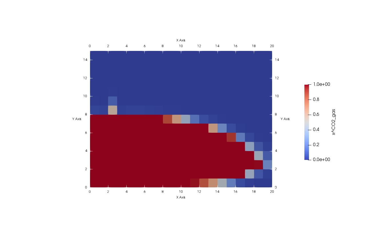
5. CO₂ injection to test aquitard integrity

Now, the sealed aquitard is tested with a CO₂-Injection into the lower CO₂-storage aquifer.

Task:

Implement a new boundary condition on the left boundary, injecting CO₂ from 2 m to 3 m from the bottom. Make sure, that the injection time for the calcium and urea is finished. You can use the predefined value gasFlux directly and divide it by the molar mass of CO₂. Run two simulations and compare them side by side by creating two input files, or overwriting the input file in the command line:

./exercise_biomin -Problem.Name biominNoUrea -Injection.ConcUrea 0

The result for the biomineralization process during the CO₂ injection should look like this:

6. Change the permeability law

Now, we want to change the way the change in permeability due to the precipitation is calculated. While the initially used Kozeny-Carman relation is widely used, another common relation is the so-called Power Law.

Task:

Implement the Power-Law relation to create a new permeability law. For this, you can copy the existing header dumux/material/fluidmatrixinteractions/permeabilitykozenycarman.hh to the folder fluidmatrixinteractions in the exercise, rename it and within the file adapt the guarding macro, the class name, and the calculations for updating the permeability. Alternatively, you can work with the pre-prepared header permeabilitypowerlaw.hh in the folder fluidmatrixinteractions, in which only the calculations for updating the permeability are left to be modified. The equation of the Power Law is defined as:

\displaystyle K = K_0 \left(\frac{\phi}{\phi_0}\right)^\eta

    const Scalar exponent = getParam<Scalar>("PowerLaw.Exponent", 5.0);

Then modify the return value, so that the reference permeability is actually updated

    return = refPerm pow(poro/refPoro, exponent);

As a special feature, we would like the exponent \displaystyle \eta=5 to be a run-time parameter read from the input file, as this allows easy modification of the parameter and potentially fit it. This is useful, as field-scale porosity-permeability relations might be quite uncertain. Adapt the input file params.input accordingly.

Finally, the header permeabilitypowerlaw.hh needs to be included in the spatial parameters header biominspatialparams.hh and the permeability law set to the new implementation of the Power Law.

    PermeabilityPowerLaw<PermeabilityType> permLaw_;

Note: As both the Kozeny-Carman and the Power-Law relation use the same parameters, there is no need to change the permeability function calling evaluatePermeability(refPerm, refPoro, poro) in biominspatialparams.hh:

    template<class ElementSolution>
    PermeabilityType permeability(const Element& element,
                                  const SubControlVolume& scv,
                                  const ElementSolution& elemSol) const
    {
        const auto refPerm = referencePermeability(element, scv);
        const auto refPoro = referencePorosity(element, scv);
        const auto poro = porosity(element, scv, elemSol);
        return permLaw_.evaluatePermeability(refPerm, refPoro, poro);
    }

What is the effect of the exchanged permeability calculation on the results, especially the leakage of CO₂? What if the exponent would be smaller, e.g. \displaystyle \eta=2, which would mean that the precipitation is less efficient in sealing the leakage? You can again run two simulations and compare them side by side by creating two input files, or overwriting the input file parameter in the command line:

./exercise_biomin -Problem.Name biominPowerLawExponent2 -PowerLaw.Exponent 2.0

7. Use tabulated CO₂ values instead of SimpleCO2

So far we have been using a simplified component for CO₂, which is based on the ideal gas law. Due to the conditions present in this exercise this is not too inaccurate, but for real applications of CO₂ storage changes to the model are required. We use tabulated data for density and enthalpy of CO₂, accessed through GeneratedCO2Tables::CO2Tables and Components::CO2 from DuMu^x.

Task:

The CO₂ component is used in the fluidsystem, which is defined in properties.hh. Replace the component SimpleCO2 with CO2 defined in dumux/material/components/co2.hh, with a CO₂ table as an additional template parameter. Use the table defined in dumux/material/components/defaultco2table.hh, noting the different namespace. Take care to include the appropriate headers.

#include <dumux/material/components/co2.hh> //!< CO2 component for use with tabulated values
#include <dumux/material/components/defaultco2table.hh> //!< Provides the precalculated tabulated values of CO2 density and enthalpy.

template<class TypeTag>
struct FluidSystem<TypeTag, TTag::ExerciseBioMin>
{
private:
    using Scalar = GetPropType<TypeTag, Properties::Scalar>;
    using CO2Impl = Components::CO2<Scalar, GeneratedCO2Tables::CO2Tables>;
    using H2OType = Components::TabulatedComponent<Components::H2O<Scalar>>;
public:
    using type = FluidSystems::BioMin<Scalar, CO2Impl, H2OType>;
};

Bonus: Paraview Magic: Compare different results using Programmable Filter

In the last step, the manual comparison of the results can be quite difficult. Paraview offers the option to use programmable python filters. To use them, make sure that two result files with different names are loaded. Mark both of them and click on Filters --> Alphabetical --> Programmable Filter. Now, a new field opens on the left side. Copy the following lines there:

S_gas_0 = inputs[0].CellData['S_gas'];
S_gas_1 = inputs[1].CellData['S_gas'];
output.CellData.append(abs(S_gas_0-S_gas_1),'diffS_gas');

Click Apply and select diffS_gas as new output. You should now see the difference between the two result files. You can also change the output to a not absolute value by changing the last line to:

output.CellData.append((S_gas_0-S_gas_1),'diffS_gas');